
|
Graphing Linear Functions Target E
|

|
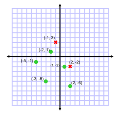
Hiram plotted seven points that satisfy the inequality \(y<-2x+1\). Tim thinks that two of the points are not solutions and marked them with red x's. Hiram thinks that all of the points work. Whom do you agree with and why?
|
A linear inequality is an inequality that involves a linear function. A linear inequality looks similar to a linear equation except for the fact that the equal sign is now an inequality symbol, which effects what the graph looks like tremendously. Observe the difference between the graphs of a linear equation versus a linear inequality with the same slope and same y-intercept.
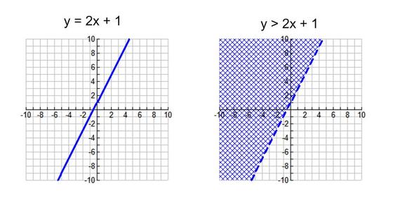
Why are the graphs so different? Try to remember the number of solutions that a more simple inequality, such as \( x > 3 \), would have. There is not just one number that can be substituted in for \( x \) that would create a true statement. The value of \( x \) could be \( 4, 5, 6, \pi \) and so on, as long as the value of \( x \) is greater than \( 3 \), as stated in the inequality. A similar thing happens when we have an inequality with two variables. There is not just one \( (x, y) \) ordered pair that would create a true statement, there are a number of possibilities that will create a true statement when substituted into the inequality. Let’s examine a few of the ordered pairs in the shaded region of the graph.
Substituting in the point \( (1, 6) \) into the inequality \( y > 2x + 1 \) we get \( 6 >2(1) + 1 \) which becomes \( 6 > 3 \), which is a true statement. \( (1, 6) \) is a solution to the inequality.
Substituting in the point \( (-7, 2) \) into the inequality we get \( 2 > 2(-7) + 1 \) which becomes \( 2 > -13 \), which is also a true statement. \( (-7, 2) \) is also a solution to the inequality.
Now you choose a point in the shaded region! What happens when you substitute the point into the inequality?
What ends up happening when graphing a linear inequality, is that the shaded region (sometimes called the feasible region) represents all the possible ordered pairs that are solutions to the inequality. The non-shaded region represents all the ordered pairs that are not solutions. So if you were to substitute any point from the non-shaded region into the inequality, it would result in a false statement. But what about the points that are on the boundary line (the dashed line in the graph above)? Substituting the point \( (2, 5) \) which is on the line into the inequality will result in a false statement. \( 5 > 2(2) + 1 \) which becomes \( 5 > 5 \), which is not true. So when graphing linear inequalities there are two different types of lines used when we draw the boundary line: dashed and solid. The inequality symbols are what determine the type of line drawn:
Where the shading occurs can also be determined by the inequality symbol as well, as long as the linear inequality is written in SLOPE-INTERCEPT form.
Now that we know the basics behind the graph of a linear inequality, let’s practice graphing a few!
Substituting in the point \( (1, 6) \) into the inequality \( y > 2x + 1 \) we get \( 6 >2(1) + 1 \) which becomes \( 6 > 3 \), which is a true statement. \( (1, 6) \) is a solution to the inequality.
Substituting in the point \( (-7, 2) \) into the inequality we get \( 2 > 2(-7) + 1 \) which becomes \( 2 > -13 \), which is also a true statement. \( (-7, 2) \) is also a solution to the inequality.
Now you choose a point in the shaded region! What happens when you substitute the point into the inequality?
What ends up happening when graphing a linear inequality, is that the shaded region (sometimes called the feasible region) represents all the possible ordered pairs that are solutions to the inequality. The non-shaded region represents all the ordered pairs that are not solutions. So if you were to substitute any point from the non-shaded region into the inequality, it would result in a false statement. But what about the points that are on the boundary line (the dashed line in the graph above)? Substituting the point \( (2, 5) \) which is on the line into the inequality will result in a false statement. \( 5 > 2(2) + 1 \) which becomes \( 5 > 5 \), which is not true. So when graphing linear inequalities there are two different types of lines used when we draw the boundary line: dashed and solid. The inequality symbols are what determine the type of line drawn:
- Dashed line: The symbols \( < \) or \( > \) are used when points along the boundary line are not solutions to the inequality.
- Solid line: The symbols \( \leq \) or \( \geq \) are used when points along the boundary line are solutions to the inequality.
Where the shading occurs can also be determined by the inequality symbol as well, as long as the linear inequality is written in SLOPE-INTERCEPT form.
- Shade above the boundary line: \( > \) or \( \geq \)
- Shade below the boundary line: \( < \) or \( \leq \)
Now that we know the basics behind the graph of a linear inequality, let’s practice graphing a few!
Graphing a Linear Inequality from Slope-Intercept Form
Graphing a Linear Inequality by Converting to Slope-Intercept Form
Graphing Linear Inequalities with One Variable
Quick Check
Graph the following inequalities:
1) \( 2x -3y > 9 \)
2) \( y \leq \frac{7}{2} \)
Graph the following inequalities:
1) \( 2x -3y > 9 \)
2) \( y \leq \frac{7}{2} \)